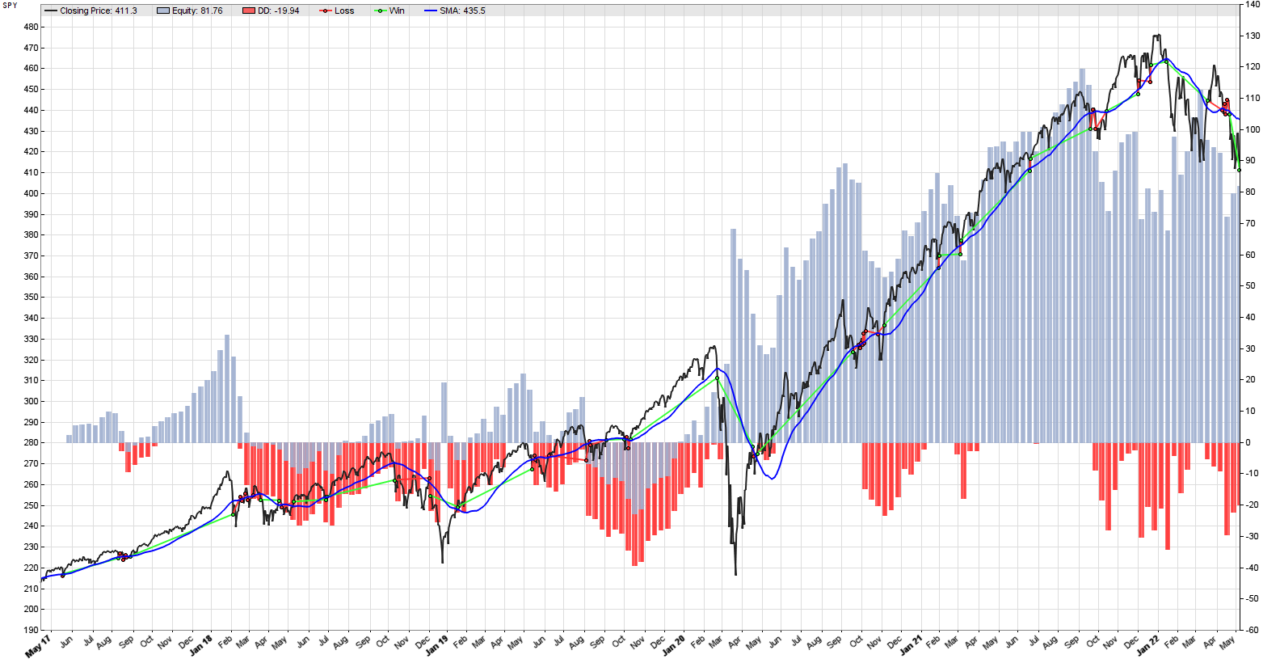
In this post, we will implement the simplest systematic trend following strategy in Zorro Trader, and we will run a back-test to measure its historical performance. The image above represents graphically the output of the strategy in a back-test. The underlying asset in this case is the SPY, an SP500 exchange traded fund (ETF). In plain English, the strategy can be expressed as follows:
- Calculate a simple moving average of a certain length. (We chose 50 days here, arbitrarily.)
- If the price of the asset crosses above the simple moving average, we will close any short positions and will go long.
- If the price of the asset crosses below the simple moving average, we will close any long positions and go short.
The rationale of this strategy is that a moving average contains less noise than the price curve, and it assumes that trends in the market tend to persist for some time. A cross of the price above de simple moving average represents a bullish signal, while a cross below is a bearish signal. The strategy is 100% of the time in the market, and switches between long and short positions according to the signals. It can’t really get any simpler than that, can it?
Implementing this strategy in Zorro Trader is extremely easy. Here is the Lite-C code:
function run()
{
	BarPeriod = 1440;

	vars price = series(priceClose());
	vars sma = series(SMA(price, 50));

	if(crossOver(price, sma)) enterLong();
	if(crossUnder(price, sma)) enterShort();
}
This is all we need in order to implement, back-test and live trade the strategy (if you chose to do so, but we strongly urge you NOT to). In order to visualize the simple moving average in the resulting image, we need to add the following line of code at the end. BEFORE the last curly brace, of course…
plot("SMA", sma, LINE, BLUE);
Honestly, it can’t really get much simpler than this! In a way, this is the “Hello, World!” program for algorithmic trading with Zorro Trader. Let’s give the code a closer look. The run() function of Lite-C is similar to the main() function in C, but with a major difference. main() gets executed only once, while run() gets executed whenever a new OHLC bar comes in, either from the broker (in live trading) or from the historical data file (in a back-test).
Talking about OHLC bars, the first variable we have to initialize is… the bar period. How long is it, in minutes? By default, Zorro Trader uses 1 minute bars, so we will set here BarPeriod to a full trading day (1440 minutes). Please note that we do not have to set a type for this variable as it is an internal variable of Zorro Trader.
Define variables
Next, we have to define and initialize two variables, on that will hold the closing prices time series, and the other one the simple moving average time series. Both these variables are series of numbers (EOD and SMA) so we will use the Lite-C vars type. Since they are time series, we will use the predefined Zorro Trader function series() to create them. This function will take as argument two other predefined functions, priceClose() and SMA().
priceClose() pulls the closing prices, and SMA() calculates a moving average on the prices. SMA() also needs a length argument, respectively how many days we want the simple moving average to span. We ask for a 50 days moving average, for no particular reason.
The following couple of lines define our trading logic. if() sets a condition, which is then checked by two Zorro Trader predefined functions: crossOver() and crossUnder(). They take as arguments the two time series that can cross, the price and the simple moving average. If either condition is true, enterLong() and enterShort() will enter positions with your broker (in live trading) or trigger performance calculations in a back-test.
Zorro Trader Output
By default, Zorro Trader plots in the output de price curve, the trades and the equity curve. In order to add the simple moving average, we use the plot() function, which takes as arguments a caption for the plotted curve ("SMA"), the time series to be plotted (sma – the simple moving average) and the line type and color. Pretty simple, clear and self explanatory… at least for programmers. And if you are not one yet, you can easily learn in the members area of our website.
Zorro Trader standard performance report
Test SimpleStrategy SPY, Zorro 2.444

Simulated account   AssetsFix
Bar period          24 hours (avg 2087 min)
Total processed     1953 bars
Test period         2017-04-28..2022-05-06 (1265 bars)
Lookback period     80 bars (23 weeks)
Montecarlo cycles   200
Simulation mode     Realistic (slippage 5.0 sec)
Avg bar             357.1 pips range
Spread              10.0 pips (roll 0.00/0.00)
Commission          0.02
Contracts per lot   1.0

Gross win/loss      301$-216$, +8448.2p, lr 117$
Average profit      16.83$/year, 1.40$/month, 0.0647$/day
Max drawdown        -44.83$ 53.1% (MAE -70.05$ 82.9%)
Total down time     62% (TAE 93%)
Max down time       121 weeks from Feb 2018
Max open margin     463$
Max open risk       4.75$
Trade volume        22579$ (4497$/year)
Transaction costs   -7.10$ spr, 0.39$ slp, 0$ rol, -1.42$ com
Capital required    498$

Number of trades    71 (15/year)
Percent winning     26.8%
Max win/loss        48.86$ / -9.59$
Avg trade profit    1.19$ 119.0p (+1582.2p / -415.6p)
Avg trade slippage  0.0055$ 0.6p (+15.3p / -4.8p)
Avg trade bars      17 (+51 / -5)
Max trade bars      109 (31 weeks)
Time in market      99%
Max open trades     1
Max loss streak     9 (uncorrelated 15)

Annual return       3%
Profit factor       1.39 (PRR 0.94)
Sharpe ratio        0.27 (Sortino 0.26)
Kelly criterion     2.26
Annualized StdDev   12.03%
R2 coefficient      0.614
Ulcer index         32.0%
Scholz tax          22 EUR

Year Jan Feb Mar Apr May Jun Jul Aug Sep Oct Nov Dec Total
2017                   1   0   1  -2   1   1   1   1    +4
2018   3  -7   0  -2  -1  -0   2   2   0  -1  -1   1    -3
2019  -1   2   1   2  -2  -1   1  -5   0  -1   2   2    -1
2020  -0   5   7  -6   3   1   4   4  -5  -1   0   3   +15
2021  -1  -0   1   4   1  -1   2   3  -6   1  -1  -2    +0
2022   1   3  -0  -2   0                                +1

Confidence level     AR   DDMax  Capital
 10%                  3%    33   489$
 20%                  3%    38   492$
 30%                  3%    41   495$
 40%                  3%    45   498$
 50%                  3%    49   501$
 60%                  3%    53   504$
 70%                  3%    57   507$
 80%                  3%    71   518$
 90%                  3%    93   535$
 95%                  3%   115   552$
100%                  3%   217   631$

Portfolio analysis  OptF  ProF  Win/Loss   Wgt%

SPY                 .999  1.39   19/52    100.0
SPY:L               .999  2.80   14/21    165.5
SPY:S               .000  0.60    5/31    -65.5
This is obviously not a very good trading strategy, but simple strategies such as this one rarely are. We are making an Annual Return of 3% with a Sharpe Ratio of 0.27. This means we are making less money than “the market” but we are taking on more risk (the benchmark here being the SP500). Examining the image above, we can easily spot the problem, which is typical for all trend following strategies. Although we are usually on the right side of almost all big trends, we get killed by a lot of small losing trades when the market moves sideways.
This observation may hold the key to further strategy improvements. Can we trade a different asset and do better? Can we filter out some of the bad trades in sideways market regimes? Or is this strategy truly hopeless? All these ideas will eventually become topics of our video courses in the members area.
by Algo Mike
Experienced algorithmic and quantitative trading professional.