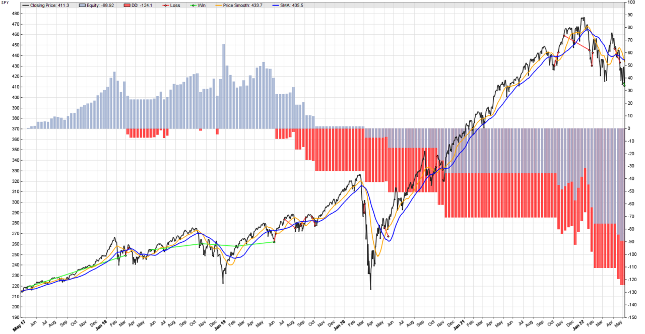
A picture is worth a thousand words, and the picture Zorro Trader produced for us (above) is not pretty. Something happened in June 2019, and after we made some profits, we started to loose money. The strategy did not change, but obviously something else did. And what changed were… the market conditions. But what exactly do we mean by that?
Changing market conditions
In general when traders say “market conditions” what they mean is either an uptrend, a downtrend or a sideways market. However, a closer examination of the picture above reveals that except for a few short periods after June 2019, the market was trending. Or, at least, it was not trending less than before June 2019. What actually did change was not the “trendiness” of the market, but something else. Before we delve into that though, it would be useful if we could look at the two back-test periods separately and examine the performance of each, separately. In order to do that, we will need to use two new Zorro Trader internal variables.
StartDate and EndDate of a Zorro Trader back-test
We suppose these two variables are self explanatory, as their names are intuitive. They do not need a type, as they are internal variables, and Zorro Trader “knows” their type already. The format of both variables is the same: yymmdd. Two digits for the year, two for the month and two for the day of the month, with no separators. A start date for a back-test on January 1, 2022 would be StartDate = 220101. An end date on May 10, 2022 would be EndDate = 220510. Can’t get any simpler than that, can it? The code of the strategy in Lite-C is below.
function run()
{
	BarPeriod = 1440;

	StartDate = 20170428;
	EndDate = 20190601;

	Stop = 0.03*priceClose();

	vars price = series(priceClose());
	vars price_smooth = series(SMA(price, 25));
	vars sma = series(SMA(price, 50));

	if(crossOver(price_smooth, sma)) enterLong();
	if(crossUnder(price_smooth, sma)) enterShort();

	plot("Price Smooth", price_smooth, LINE, ORANGE);
	plot("SMA", sma, LINE, BLUE);
}
Equity curve on SPY from April 28, 2017 to June 1, 2019
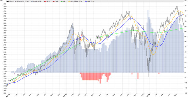
This picture shows clearly that our simple systematic strategy was profitable during this period. There was only one bad trade in March 2018, a short that worked against us, and we got stopped out. As it happens sometimes, even if we weren’t stopped out of it, it was still a bad short. The exit signal triggered above the entry price. But we would have lost less money if we followed the crossover exit signal than by getting stopped out. The stop loss didn’t really help here.
Performance analysis
Test WithStopLoss SPY, Zorro 2.444

Simulated account   AssetsFix
Bar period          24 hours (avg 2096 min)
Total processed     910 bars
Test period         2017-04-28..2019-05-31 (525 bars)
Lookback period     80 bars (23 weeks)
Montecarlo cycles   200
Simulation mode     Realistic (slippage 5.0 sec)
Avg bar             213.0 pips range
Spread              10.0 pips (roll 0.00/0.00)
Commission          0.02
Contracts per lot   1.0

Gross win/loss      42.75$-7.51$, +3524.1p, lr 42.37$
Average profit      16.87$/year, 1.41$/month, 0.0649$/day
Max drawdown        -10.56$ 30.0% (MAE -37.56$ 106.6%)
Total down time     21% (TAE 77%)
Max down time       17 weeks from Mar 2018
Max open margin     260$
Max open risk       7.93$
Trade volume        1240$ (594$/year)
Transaction costs   -0.50$ spr, 0.0000005$ slp, 0$ rol, -0.1000$ com
Capital required    273$

Number of trades    5 (3/year)
Percent winning     80.0%
Max win/loss        30.43$ / -7.51$
Avg trade profit    7.05$ 704.8p (+1068.8p / -750.9p)
Avg trade slippage  0.0000001$ 0.0p (+4.0p / -15.8p)
Avg trade bars      95 (+117 / -6)
Max trade bars      208 (60 weeks)
Time in market      90%
Max open trades     1
Max loss streak     1 (uncorrelated 1)

Annual return       6%
Profit factor       5.69 (PRR 1.42)
Sharpe ratio        0.59 (Sortino 0.54)
Kelly criterion     5.13
Annualized StdDev   11.53%
R2 coefficient      0.209
Ulcer index         44.1%
Scholz tax          9 EUR

Year Jan Feb Mar Apr May Jun Jul Aug Sep Oct Nov Dec Total
2017                   1   1   2   0   2   2   3   1   +11
2018   5  -3  -4   0  -1   1   3   3   1  -3  -2   8    +8
2019  -7   2   2   4  -7                                -6

Confidence level     AR   DDMax  Capital
 10%                  6%     5   266$
 20%                  6%     5   267$
 30%                  6%     6   268$
 40%                  6%     7   268$
 50%                  6%     7   269$
 60%                  6%     8   269$
 70%                  6%     8   270$
 80%                  6%     9   271$
 90%                  6%    11   273$
 95%                  6%    15   278$
100%                  6%    22   287$

Portfolio analysis  OptF  ProF  Win/Loss   Wgt%

SPY                 .999  5.69    4/1     100.0
SPY:L               .1000  ++++    3/0    114.6
SPY:S               .000  0.31    1/1     -14.6
Conclusions
This is not a bad result by any measure. An Annual Return of about 6% with a Sharpe Ratio of 0.59 is pretty OK for such a simple strategy. However, in order to understand what went wrong after June 2019, we need to analyze the second period of our back-test, which we will do in our next post. Learn more about Zorro Trader and the StartDate and EndDate variables from the video courses in our members area!
by Algo Mike
Experienced algorithmic and quantitative trading professional.